macro e11(u) (dx(u#1)) // $\varepsilon_{11}$
macro e22(u) (dy(u#2)) // $\varepsilon_{22}$
macro e12(u) ((dy(u#1) + dx(u#2))/2.0)
macro div(u) (dx(u#1) + dy(u#2))
int i=0;
real t=0;
real nu = 1.0/400.0;
real dt=0.1; // time step
int imax=100; // max iteration steps
int iplt0=imax/40; // interval for plot
int iplt1=imax/10; // interval for ps file
real alpha=1.0/dt;
int wall=1, slide=2, inflow=4, outflow=5;
border ba(t=0,1.0){x=t*5.0-1.0;y=-1.0;label=slide;};
border bb(t=0,1.0){x=4.0;y=2.0*t-1.0;label=outflow;};
border bc(t=0,1.0){x=4.0-5.0*t;y=1.0;label=slide;};
border bd(t=0,1.0){x=-1.0;y=1.0-2.0*t;label=inflow;};
border cc(t=0,2*pi){x=cos(t)*0.25;y=sin(t)*0.25;label=wall;};
mesh Th=buildmesh(ba(30)+bb(30)+bc(30)+bd(30)+cc(-30));
fespace Vh(Th,[P2,P2]),Qh(Th,P1),Xh(Th,P2);
Vh [u1,u2],[v1,v2],[up1,up2];
Qh p,q;
Xh psi,phi,phii;
problem NS([u1,u2,p], [v1,v2,q],solver=UMFPACK,init=i) =
int2d(Th)( // $\int_{\Omega}\{$
alpha * (u1*v1 + u2*v2) // $\frac{1}{\delta t}(\vec{u}\cdot \vec{v})$
+ nu*2.0*(e11(u)*e11(v)+2.0*e12(u)*e12(v)+e22(u)*e22(v))
- div(v)*p-div(u)*q //$-p\textrm{div}\vec{v}-q\textrm{div}\vec{u}$
- p*q*1.e-10 ) // $-\epsilon pq$
- int2d(Th)( alpha * convect([up1,up2],-dt,up1)*v1
+ alpha * convect([up1,up2],-dt,up2)*v2 )
+ on(slide,u2=0)
+ on(inflow,u1=1.0-y*y,u2=0)
+ on(wall,u1=0,u2=0);
phii = y-y*y*y/3.0;
problem streamlines(phi,psi,solver=Crout,init=i) = // from cavity.edp
int2d(Th)(dx(phi)*dx(psi)+dy(phi)*dy(psi))
- int2d(Th)((dx(u2)-dy(u1))*psi)
+ on(slide,phi=phii)
+ on(inflow,phi=phii)
+ on(wall,phi=0);
real area = int2d(Th)(1.0);
real meanp;
[u1,u2] = [0,0];
load "webplot"
for ( i = 1; i <= imax; i++) {
t=dt*i;
[up1,up2]=[u1,u2];
NS;
meanp = int2d(Th)(p) / area; p = p - meanp; // $\int_{\Omega}p^{n}\, d\Omega=0$
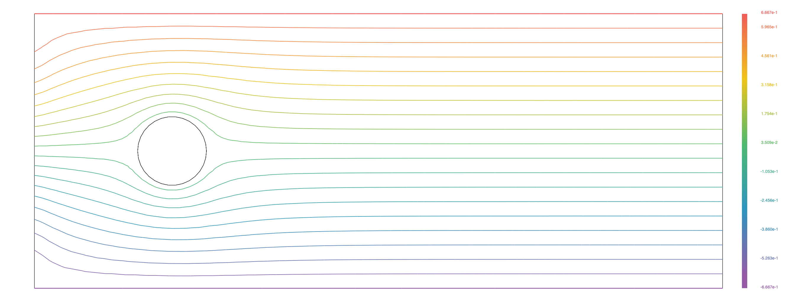
streamlines;
webplot(phi,Th,cmm="Streamlines t="+t);
}
server();